How to Calibrate a Citywide Traffic Model in PTV Visum

Traffic model calibration depends on more than matrix adjustment. A missing link, a mis-coded turn, or a poorly placed zone connector can send assigned trips down the wrong route. So can a traffic count attached to the wrong road segment. If we adjust demand before diagnosing these issues, a local improvement can conceal a network error.

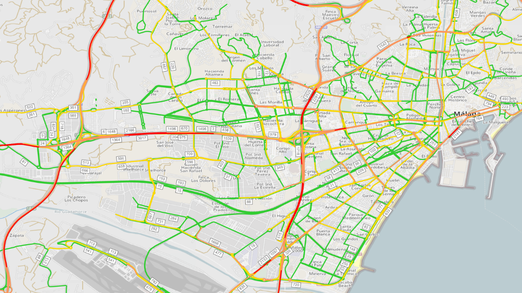
In Málaga, Spain, our team at SANVI Consulting built and calibrated a static macroscopic model of private-car traffic in PTV Visum for two one-hour peak periods: 8:00-9:00 a.m. and 2:00-3:00 p.m.

The work followed a sequence other modelers can adapt: define a network large enough to represent route alternatives, check zones and connectors, prepare observed counts, then compare assigned and observed flows.

This article explains how we diagnosed mismatches, assessed model fit with the GEH statistic, and checked the calibrated base before using it to test future scenarios.

Model beyond the project area

The project began in a defined area of Málaga. We extended the model across the city’s road network and key metropolitan connections to capture wider traffic shifts.

A change in one district can shift traffic onto parallel routes elsewhere. A model that ends near the project area may miss those shifts, while metropolitan connections give the assignment more routes to consider. The model covers private-car traffic only.

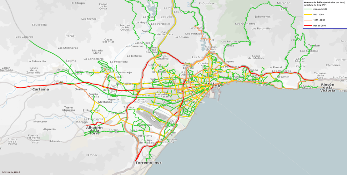
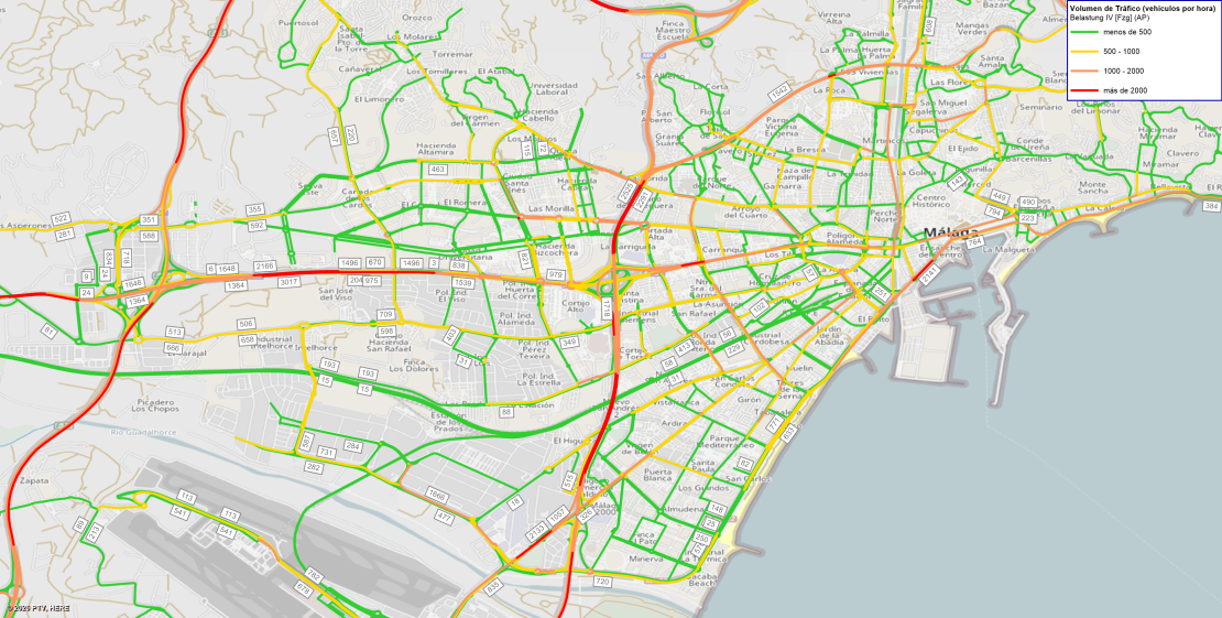
Traffic model calibration: network and zones

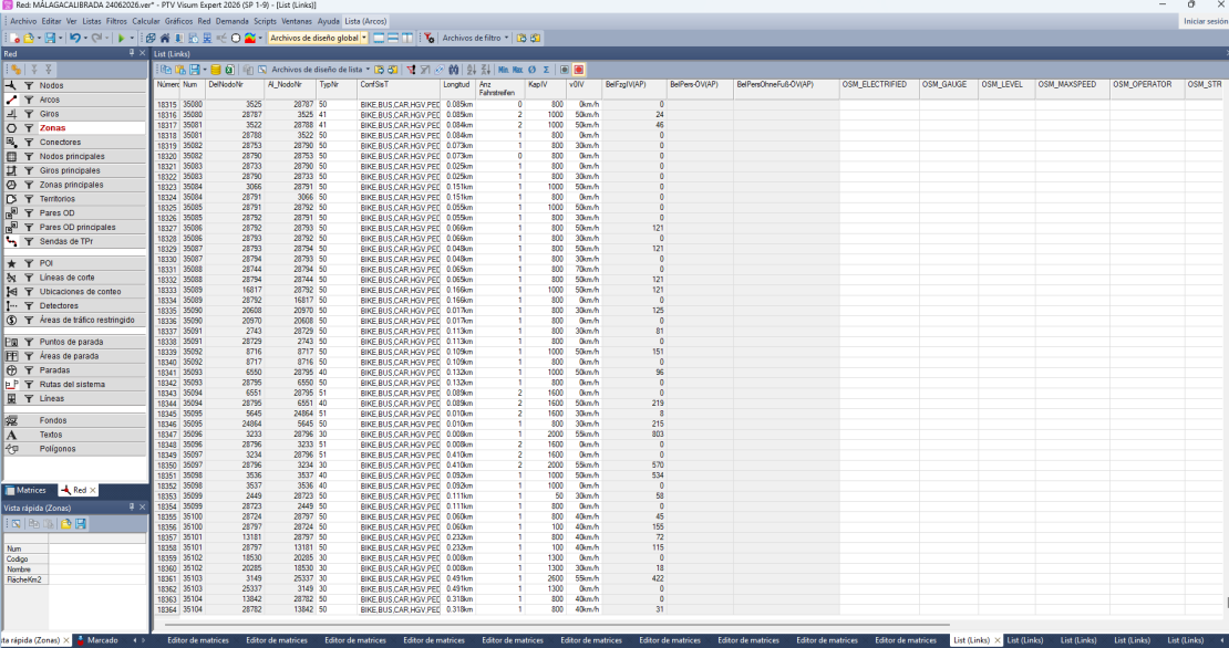
We built the road network from OpenStreetMap and information from the City of Málaga, then reviewed it manually, link by link. We checked road hierarchy, lanes, direction, turn movements and restrictions, intersection configuration, and connectivity. We also reviewed secondary roads, speeds, and capacities.

The model used 236 transport zones from the City’s 2024 mobility indicators study: 231 urban and five external.

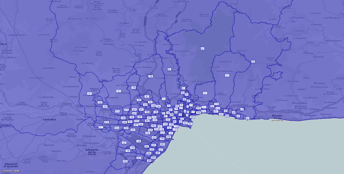
Zone connectors link each zone to the road network. Their placement affects how trips access the network, so we checked them alongside links and intersections.

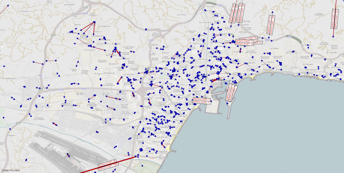
We used static macroscopic assignment with iterative user equilibrium and volume-delay functions, assigning each peak-hour matrix separately. As a road becomes more congested, its modeled travel cost rises, and some traffic may shift to other routes over successive iterations.

Each assignment represents equilibrium flows for one defined hour; it does not simulate minute-by-minute traffic changes. This distinction matters when choosing a model for a planning question and interpreting the results.

Prepare demand and counts

The same study provided origin-destination matrices for the 8:00-9:00 a.m. morning peak and the 2:00-3:00 p.m. afternoon peak. The matrices represented person trips, which we converted to private-car trips using an average occupancy of 1.35 people per vehicle.

The City provided directional hourly counts from 565 locations. We selected count data from May 7-9, 2025, considered representative of ordinary weekday conditions.

We screened outliers and readings inconsistent with road capacity, compared neighboring stations, and checked each count location against the model network. We retained 452 locations (out of 565) as control points.

Diagnose before adjusting demand

We calibrated the model by reviewing the network and demand iteratively. Checks included connectivity, secondary roads, turns, zone connectors, speeds, capacities, and the spatial distribution of trips.

We also developed a tool to compare observed counts with assigned volumes exported from PTV Visum and calculate fit indicators at each control point. The tool quickly highlighted areas with the largest discrepancies, helping us investigate causes and repeat assignments.

After adjusting the network, we found an overall demand deficit. We increased the morning and afternoon matrices by 2.81% and 3.95%, respectively.

When observed counts and assigned volumes differ, we first check that each count is linked to the correct road segment and travel direction. Next, we review nearby connections, turns, speeds, capacities, and counts. We adjust demand only when these checks indicate a demand issue.

Assess model fit

We compared assigned and observed flows at all 452 control points using the GEH statistic. During the morning peak (8:00-9:00 a.m.), 309 points (68.4%) had GEH below 5. During the afternoon peak (2:00-3:00 p.m.), 293 points (64.8%) did.

The project also used reference thresholds of at least 90% of points below GEH 10, with all remaining points below GEH 12. The reported results show 96.3% of morning points and 96.2% of afternoon points below GEH 10. In both periods, all remaining points had GEH below 12.

Test future scenarios

A calibrated base model lets planners compare how changes in demand, road capacity, infrastructure, or urban development may redistribute vehicle trips.

The 8:00 a.m. matrix for 2049 was used to assess how the city might respond after construction of a trip-attracting or trip-generating element.

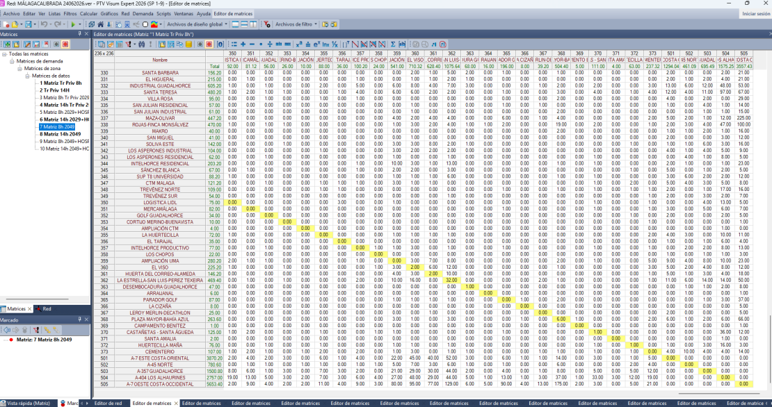
A calibrated base is a starting point, not a guarantee of accurate future forecasts. Long-range results depend on assumptions about land use, trip generation, the network, and travel behavior. State those assumptions clearly and compare alternatives consistently.

Traffic model calibration is structured diagnosis: check network and zone access, understand how counts were selected, verify trip-conversion assumptions, and adjust network and demand iteratively.

In this Málaga project, PTV Visum provided the framework for representing the road network and assigning traffic. Credible conclusions still depend on transparent inputs and comparison with observed traffic.

Get free PTV Visum demo